Topics in Model Performance
References
Bayesian Analysis with Python: Introduction to Statistical Modeling and Probabilistic Programming with PyMC3 and ArViz, 2nd Edition
You may have heard the saying
All models are wrong, but some are useful
This aphorism is attributed to the British statistician George E.P. Box. The implication of this is that models are supposed to represent reality but they rarely do in full fidelity. However, some models can provide useful insight while others add little value to what we already know, or worse provide us misleading information.
So how do we determine if our model can be trusted? In Machine Learning, we resort to Cross-Validation to provide us with a sense of certainty about a model’s ability to generalize to unseen data. Let us look at some other measures with roots in information theory to assess the predictive ability of our models.
Underfitting vs. Overfitting
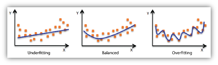
Most folks have by now heard of underfitting and overfitting a model. Simpler models should be preferred but not at the cost of accuracy. An overfit model, on the other hand, may not generalize well on new data. We can measure how well a model fits the data using the \(R^2\) metric which measures the proportion of explained variance.
If we use the example of linear regression and start with a first order polynomial regression to explain the data, we may find that the data may not be adequately captured. This is referred to as underfitting. We may have to incrementally increase the complexity of the model by increasing the order of the polynomial. Past a certain point, however, the model starts overfitting to the data. What this means is that the model simply used its representational power to memorize the data and will perform poorly on new data that is fed into the model (\(R^2\) too high).
We want a model that has found that balance between being underfit and overfit, this trade-off is often referred to as the bias-variance trade-off. Bias is the error in the data resulting from its inability to accomodate the data. The model does not have the representational power to capture all the variations and patterns in the data. Variance is the error resulting from the sensitivity of the model to the data, which usually results from too complex of a model. Regularization is often used for this reason to reduce the complexity in a regression model (or neural network) by minimizing the number of coefficients.
\(R^2\) and Explained Variance
What does it do?
\(R^2\) is a goodness-of-fit measure that tells you how well the data fits the model that we created. More pedantically, it explains the proportion of variance in the outcomes that the independent variables explain.
Derivation
If we observe data given by \(y_i\) such that the fitted model predicts \(f_i\) for each point i, we can write the mean of all the observed data, given by \(y_{mean}\) as
Total sum of squares, which is proportional to the variance of the data, is
The residual sum of squares (also called the error) is defined as
Now, \(R^2\) is defined as
How do we interpret this?
\(R^2\) is 1 for a model that perfectly fits the observed data, i.e. \(f_i = y_i\) for all i.
If the model predicts \(y_{mean}\) always then \(SS_{res} = SS_{tot}\) and \(R^2 = 0\), this indicates a baseline model to which all other models can be compared.
Any model that performs worse than the baseline model will have a negative \(R^2\) score.
Explained Variance
The term \(\dfrac{SS_{res}}{SS_{tot}}\) is also called Unexplained Variance. Therefore
\(R^2 = 1 - Unexplained Variance\)
or
\(R^2 = Explained Variance\)
Measures for Predictive Performance
Accuracy of the model can be measured by the following methods:
1. Cross-Validation
Here we divide the data into non-overlapping subsets and perform training and validation on the different subsets. Depending on how we perform this Cross-Validation, it can be called K-fold Cross-Validation or leave-one-out Cross-Validation (LOOCV). In K-fold Cross-Validation we divide the data into ‘K’ folds or subsets, perform training of the model on k-1 folds while the model performance is assessed on the 1 fold that was left. We iteratively select each fold to be the test fold while the others become the training folds.

If the number of folds is equal to the number of data points, we have Leave-One-Out Cross-Validation.
2. Information criteria
Reference
A number of ideas that are firmly rooted in information theory help us to quantify how well a model performs.
Log-likelihood (Log predictive density) and deviance
Akaike Information Criterion (AIC)
Widely Applicable Information Criterion (WAIC)
Deviance Information Criterion (DIC)
Bayesian Information Criterion (BIC)
For (2) to (5),
They take the form of the equation with two terms given by
\[metric = model\;fit + penalization\]The model fit is measured using the log likelihood of the data given model parameters (could be a pointwise estimate, or could use the full posterior distribution)
Lower values imply a better fit
AIC, BIC and DIC use the joint probability of the data, whereas WAIC computes the pointwise probability of the data. In the following, we assume the model parameters are independent, thereby the joint probability is the same as the product of the pointwise estimates.
Log-likelihood and Deviance
Reference
These terms are used to measure the error in our model with regards to the data that the model is trying to fit. Most folks are familiar with the Mean Squared Error (MSE) given by
Log-likelihood (Log predictive density)
While this is a perfectly acceptably way of measuring error especially if the likelihood is a normal distribution, a more theoretically justified way to measure the performance of a model is using the log-likelihood function.
If the likelihood function is a Normal, the log-likelihood is proportional to the MSE.
Deviance
Deviance is two times the log-likelihood of the model subtracted from the log-likelihood of a saturated model. A saturated model is one that has overfitted to the point that it fits the observed data perfectly. It can be rewritten to emphasize that the range of values are now from 0 to \(\infty\).
Why use the Deviance over the Log-likelihood?
Note that the likelihood function \(p(y_i | \theta)\) takes values from 0 for no fit to 1 for a perfectly fit model. This results in the log-likelihood function taking values from \(- \infty\) to 0. Multiplying the log-likelihood function by -2 results in a number that is interpretable similar to the MSE.
Poorly fit models have large positive values
A perfectly fit model has a value of 0.
Complex models will have lower deviance values on the training set (in-sample data), and this needs to be penalized when comparing models. This is related to model overfitting that we talked about earlier.
A Note on MLE
Maximum Likelihood Estimation (MLE) is based on the notion of estimating the parameters \(\theta\) that maximize the the probability \(\sum_1^n p(y_i | \theta)\). While there are other methods to do the same, with a large enough sample size MLE is the most efficient estimator for the distribution parameter \(\theta\). Also, as sample size increases the estimated parameter tends to the true parameter and the error becomes normally distributed.
A disadvantage of the MLE arises when you have non-regular distributions, i.e. distributions whose parameters are constrained by the observed values. For such distributions, a maximum likelihood may not exist. Similar problems can occur in cases where multiple maxima exist.
Posterior Predictive Distribution to Estimate Predictive Accuracy
This also sets the stage to be more Bayesian by utilizing the posterior predictive distribution. This allows us to measure the model’s probability of generating the new data i.e. \(p(y_{new} | y)\). This can be interpreted as asking “What is the probability of seeing the new out-of-sample-data, given the model that was trained on the in-sample data?”. The predictive accuracy can be written as
where \(p(\theta | y)\) is the posterior distribution for \(\theta\) and we integrate over the entire distribution of \(\theta\). Now this is simply the expectation of \(p(y_{new} | \theta)\) over the posterior distribution of \(\theta\). In simple terms, it is the average of all the probabilities of seeing \(y_{new}\) calculated over all possible values of \(\theta\).
This has the following steps
Draw a \(\theta_i\) from the posterior distribution for \(\theta\)
Given the value of \(\theta_i\) how likely are you to see \(y_{new}\), or compute \(p(y_{new} | \theta_i)\)
Repeat (1) and (2) several times to compute the expectation of \(p(y_{new} | \theta)\)
This is also computed using the log frequently as
Akaike Information Criterion (AIC)
The AIC is derived from the world of Frequentist statistics and does not use the posterior distribution. Therefore, instead of integrating over the posterior, it uses the MLE estimate for \(\theta\). The term \(E [ p(y_{new} | \theta) ]\) is now replaced with \(p(y_{new} | \theta_{mle})\).
Here \(n_{parameters}\) refers to the number of parameters in the model and \(\theta_{mle}\) is the MLE estimate of \(\theta\). We want a model with a lower AIC and the second term is intended to penalize complex models by increasing the value of AIC. Since this does not use the posterior distribution, it does not take into account any information regarding the uncertainty of the parameter.
Bayesian Information Criterion (BIC)
The BIC is very similar to the AIC (and in fact not very Bayesian at all). The first term is identical to that in the AIC, however the bias correction term now incorporates the number of samples as well.
Deviance Information Criterion (DIC)
The DIC is a more Bayesian alternative that uses the posterior mean point estimate \(\theta_{Bayes}\) instead of the MLE estimate. Here \(\theta_{Bayes}\) is the expected value of \(\theta\).
Widely Applicable Information Criterion (WAIC)
Reference
The Widely Applicable Information Criterion or WAIC is a Bayesian extension to the AIC. The derivation for the log pointwise predictive density is similar to what we covered above, but is replicated here to keep it consistent with the paper referenced.
Log pointwise predictive density (lppd)
The predicted value of a new data point \(y_{new}\) can be defined
If we take the log of both sides we get
where \(p_{post}(\theta)\) is the posterior distribution of \(\theta\) obtained by training our model. This is the predictive fit of the new point. If we have a number of new data points i=1,…n we can write the following for the log pointwise predictive density for a model using the new data
In practice, the inner integral over \(\theta\) is computed using an average over possible values of \(\theta\) (sampled) denoted as \(\theta_S\).
Now suppose we don’t have a holdout set \(y_{new}\) and we compute the lppd over our training set, that is not a good measure for future performance of the model. So the WAIC adds a term to correct for this overestimated performance. This correction measures the variance of the log-likelihood for each element of y computed over the different samples of \(\theta_S\). This correction can be seen as a type of penalization intended to reduce the number of parameters since more model parameters imply larger spread or variance of the posterior.
WAIC is now defined as the sum of the two terms above
A Qualitative Discussion
The AIC may not work as well for more complex models since this just uses the number of parameters to penalize the model
It is worth emphasizing here that all the metrics/methods above, with the exception of Cross-Validation (with a test set) use in-sample data to assess out-of-sample performance. This is analogous to using the training set instead of a test set to evaluate the model performance in Machine Learning. However, unlike what is normally performed in Machine Learning, we apply a bias correction to correct for the error introduced by estimating the performance on the in-sample data. However, Cross Validation eliminates the need for this error correction altogether if a test set is used.
AIC and DIC are easier to compute but they are not fully Bayesian unlike the WAIC. However, the WAIC is more computationally intensive to calculate.
Cross-Validation can be made Bayesian by computing the log posterior density. However, this becomes quite expensive to compute compared to the other techniques.
Entropy and KL Divergence
Reference
I am using summation in the examples below assuming discrete distributions. This can be replaced by the integral for continuous distributions.
Entropy
If there is a random discrete variable ‘x’ with a probability distribution given by P(x), the entropy of the random variable ‘x’ is a measure of information uncertainty, which can be computed as
where a larger value of entropy indicates higher uncertainty. Geometrically, we can visualize this as the distribution having a larger spread. While is easy to equate this with variance, there are examples such as a Bimodal Gaussian distribution where increasing the variance does not increase the entropy. Entropy is a measure of the mass of probability density around a point whereas variance measures how far the probability mass extends from the mean. It is possible to have two narrow modes that are far apart which would indicate a high variance but low entropy due to the relative certainty of the values (around the narrow modes).
Entropy is a useful way to define priors since a prior with high entropy can be used as an uninformative prior. Given certain constraints on the parameter values, the following can be used as priors for those parameters.
No constraints - Uniform distribution
Positive mean with regions of high density - Exponential distribution
Fixed variance - Normal distribution
Two outcomes with a fixed mean - Binomial distribution
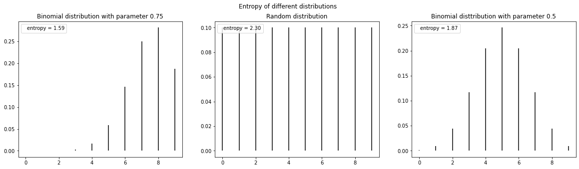
The following code shows the entropy of different distributions
# Example from [1]
import numpy as np
from scipy import stats
from matplotlib import pyplot as plt
np.random.seed(912)
x = range(0, 10)
q = stats.binom(10, 0.75)
q2 = stats.binom(10, 0.5)
r = stats.randint(0, 10)
true_distribution = [list(q.rvs(200)).count(i) / 200 for i in x]
q_pmf = q.pmf(x)
q2_pmf = q2.pmf(x)
r_pmf = r.pmf(x)
fig, ax = plt.subplots(1,3, figsize=(20,5))
ax[0].vlines(x, 0, q_pmf, label=f'entropy = {stats.entropy(q_pmf):.2f}')
ax[1].vlines(x, 0, r_pmf, label=f'entropy = {stats.entropy(r_pmf):.2f}')
ax[2].vlines(x, 0, q2_pmf, label=f'entropy = {stats.entropy(q2_pmf):.2f}')
ax[0].set_title('Binomial distribution with parameter 0.75')
ax[1].set_title('Random distribution')
ax[2].set_title('Binomial disttribution with parameter 0.5')
fig.suptitle("Entropy of different distributions")
stats.entropy(true_distribution)
#ax[idx].set_xticks(x)
ax[0].legend(loc=2, handlelength=0)
ax[1].legend(loc=2, handlelength=0)
ax[2].legend(loc=2, handlelength=0)
<matplotlib.legend.Legend at 0x7fb442937df0>
UNGRADED EVALUATION (15 mins)
Try the above with different parameters for
The Binomial distribution
The Poisson distribution
KL Divergence
KL Divergence is similar to the concept of entropy except that it is used to compare the similarity and closeness of two distributions. It is defined for two discrete distributions as
The value of the KL Divergence varies from 0 for identical distributions to infinity depending on the dissimilarity between the distributions. It is important to understand that this is not a distance metric as it is not symmetric, since
The Jensen Shannon Divergence is the symmetric version of the KL Divergence
The KL Divergence \(KL(p||q)\) can be seen as the difference of two entropies
where the first term is the entropy of ‘p’ and the second term is the cross-entropy between ‘p’ and ‘q’.
The KL Divergence is commonly used in Machine Learning to learn a distribution. If the true distribution was available, the proposed distribution can be optimized to make it as close to the true distribution as possible.
from scipy.stats import entropy

print("KL Divergence between the true distribution and the uniform distribution ",entropy(true_distribution, r_pmf))
print("KL Divergence between the true distribution and the q distribution ",entropy(true_distribution, q_pmf))
print("KL Divergence between the true distribution and the q2 distribution ",entropy(true_distribution, q2_pmf))
KL Divergence between the true distribution and the uniform distribution  0.7394593875511319
KL Divergence between the true distribution and the q distribution  0.009657896086383405
KL Divergence between the true distribution and the q2 distribution  1.276465607901914
UNGRADED EVALUATION (1 hr)
Write Python code to compute the KL divergence between two distributions. Use two normal discrete distributions a and b with different mean and variance. Note how the KL divergence changes as the number of samples in the distribution increases.
Compute the KL Divergence between a and b - KL(a||b)
Compute the KL Divergence between b and a - KL(b||a)
Compute the KL Divergence between a and itself
Compute the KL Divergence between a and the shifted version of a. Note how the KL Divergence varies as the shifted version moves away.
Model Averaging
Sometimes, model selection may not the most appropriate solution for our problem, e.g. when none of the individual models provide satisfactory performance. Or, as mentioned below when we want to utilize the variance associated with the different models as a measure of uncertainty. In these cases we may want to resort to model averaging.
Pseudo Bayesian Modeling Averaging
Using Stacking to Average Bayesian Predictive Distributions
When there are several models that one can chose from, it is tempting to pick the one with the best performance (depending on how we define performance). However, in doing so we are ignoring the uncertainty information provided by the other models. One way to mitigate this uncertainty is by performing model averaging. The meta-model obtained by using a weighted average of all the models can be used to make predictions. One way that this averaging is done is by computing the weights similar to using a softmax formula
where \(dE_i\) is the difference in the WAIC value of the i’th model compared to the model with the lowest WAIC.
Any Information Criterion metric can be used in this equation such as the AIC. Averaging the models using the weights computed this way is called pseudo Bayesian Modeling Averaging.
Stacking
Another technique that was proposed recently is the stacking of predictive distributions. The idea behind this is to combine models such that you minimize the divergence between the weighted metamodel and the true model. When a logarithmic score is used, similar to a KL Divergence, the following equation can be used
where n is the number of data points and \(M_k\) is the k’th model and \(w_k\) is the weight applied to the k’th model. \(y_{-i}\) is every element in y except \(y_i\). The term \(p(y_i | y_{-i}, M_k)\) corresponds to the predictive probability density using a Leave-One-Out Cross-Validation (LOOCV) procedure. The goal is to select the combination of weights that maximizes the probability of seeing \(y_i\), thereby giving us the ideal metamodel that minimizes the divergence, to the best of our knowledge, based on the data available. Note here that argmax is computed over ‘w’ as opposed to ‘n’ as it listed in some resources.
GRADED EVALUATION (30 mins)
Underfitting is bad because
a. It cannot capture complex behavior and will have inherent error (
b. The predicted value is always less than the true value
Overfitting is bad because
a. The model that is overfit will learn noise
b. The model is too big
Variance of a model is related to
a. A model’s ability to adapt its parameters to training data
b. The sensitivity of the model to the inputs
AIC is a primarily a non-Bayesian metric
a. True
b. False
KL Divergence is a distance metric
a. True
b. False
The symmetric version of the KL Divergence is
a. Jenson Button Divergence
b. Jensen Shannon Divergence
Entropy is a measure of
a. Information symmetry
b. Information uncertainty
The WAIC is the Bayesian extension to the AIC
a. True
b. False
For Deviance of models, a well-fit model has a value
a. Infinity
b. Close to 0
The value of \(R^2\) for a model that perfectly fits the data is
a. 1
b. 0