Probability - II
Addition rules
Addition rules deal with unions (\(\cup\)) of events. These can be thought of as OR probabilities.
(\(\bigcup\) - non-repeating superset, \(\bigcap\) - common elements)
or when A and B are mutually exclusive
In the figure below, A represents a case where events in the two shaded regions are mutually exclusive, ie there are no overlapping areas. In B, the overlapping area is the intersection (\(\cap\)) of the two areas.

Multiplication rules
Multiplication rules deal with intersections (\(\cup\)) of events. These can be thought of as AND probabilities.
(\(\cup\) - non-repeating superset, \(\cap\) - common elements)
Dependent
$\(P(A \cap B) = P(A) \ast P(B|A)\)$
Independent
$\(P(A \cap B) = P(A) \ast P(B)\)$
Mutually exclusive
$\(P(A \cap B) = 0\)$
Conditional, Independent, disjoint, exchangeable
Conditional
$\(P(A|B) = \frac{P(A,B)}{P(B)}\)$
Independent
$\(P(A,B) = P(A) \ast P(B)\)$
Disjoint
$\(P(A,B) = 0\)$
Exhangeable
$\(P(A then B) = P(B then A)\)$
Factoring joint probabilities
Given a joint probability, we often need to simplify to get to some tractable or known distribution. We can do this via the rules given above and the chain rule.
Random variable
Random variables are (often) real-valued functions mapping outcomes to a measurable space. In set notation, this looks like:
This mapping defines the probability giving by X in a measurable set as:
Random sample, experiment, trial
Random sample = unbiased realization of outcomes
Random experiment = an activity with an observable result
Trial = 1 or more experiments
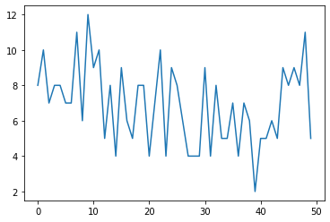
In the figure and table below, we are plotting and tabulating the results from the roll of two dice. We did not define the experiment up front, but will do so now for clarity.
Experiment = throw 2 dice 500 times
Trial = in this case, there was a single trial of the experiment
Random sample = we have 500 realizations of two dice being thrown
Note, due to how random numbers are generated and are used to get the die rolls, we sampled with replacement into a long 1000 long list. We then pulled the list into two sequences with every other 1 being die1 vs die2. We could have done this in a for loop rolling both dice in each iteration. Based on how randon numbers are generated, this would have resulted in the same sequence of die rolls.
## look at the first 10 dice throws
print(df.head(n=10))
# view the first 50 throws
tplot = df['dots'].head(n=50).plot()
Data generating mechanism
This is the actual process we are trying to model. In the case of the dice, it was the throwing and counting of dots where we are looking to learn (and use) a statistical model of outcome probabilities. In a count toss experiment, it is the binary outcome of heads or tails.
GRADED EVALUATION (15 mins)
Two events A and B are independent, their joint probability is given as:
a. \(P(A,B) = P(A) \ast P(B)\)
b. \(P(A,B) = 0\)
Given both a fair coin and 6-side die, we know P(coin) = 1/2 and P(die) = 1/6 for any landing of the coin and die. What is the joint probability for any of the possible combinations of outcomes?
a. \(P(A,B) = P(A) \ast P(B) = \frac{1}{12}\)
b. \(P(A,B) = P(A) + P(B) - P(A or B) = \frac{1}{3}\)
In a certain game, you are given \(P(A,B) = 1/12, P(A) = 1/2\) and \(P(B) = \frac{1}{4}\). Are the events independent?
a. no
b. yes
For the last question, what is \(P(A|B)\)?
a. \(P(A|B) = P(A,B)/P(B)\)
b. 0
Two events are said to be exchangeable if
a. The order of occurrence doesn’t matter.
b. They are independent.
A random variable is:
a. A real valued fuction mapping outcomes to the real number line.
b. A real valued fuction mapping occurrence of events to the real interval [0,1].
The marginal distribution of X for \(f(x,y) = \frac{1}{4}xy\text{, x,y }\in [0,2]\) is
a. \(\frac{1}{2}x\)
b. \(\frac{1}{2}y\)