Centered vs. Non-centered Parameterization
When there is insufficient data in a hierarchical model, the variables being inferred end up having correlation effects, thereby making it difficult to sample. One obvious solution is to obtain more data, but when this isn’t possible we resort to reparameterization by creating a non-centered model from the centered model.
Centered Model
And we try to fit the two parameters for \(\mu\) and \(\sigma\) directly here.
Non-centered Model
import numpy as np
import pymc3 as pm
import matplotlib.pyplot as plt
from matplotlib import rcParams
from scipy.stats import norm, halfcauchy, halfnorm
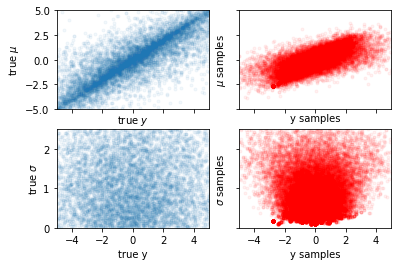
def centered_model():
# generate data
np.random.seed(0)
n = 1
m = 10000
mu = norm.rvs(0, 3, m)
sigma = halfnorm.rvs(0, 2, m)
y = norm.rvs(mu, sigma, (n, m))
# set up model
with pm.Model():
mu_ = pm.Normal("mu", 0, 1)
sigma_ = pm.HalfNormal("sigma", 1)
y_ = pm.Normal("y", mu_, sigma_, shape=n)
# sample and save samples
trace = pm.sample(m, chains=3)
mu_samples = trace["mu"][:]
sigma_samples = trace["sigma"][:]
y_samples = trace["y"].T[:]
sc = 5
fig, axes = plt.subplots(2, 2, constrained_layout=False, sharex=True)
ax = axes[0, 0]
ax.scatter(y[0], mu, marker=".", alpha=0.05, rasterized=True)
ax.set_xlim(-sc, sc)
ax.set_ylim(-sc, sc)
ax.set_ylabel("true $\mu$")
ax.set_xlabel("true $y$")
ax = axes[0, 1]
ax.scatter(y_samples[0], mu_samples, marker=".", alpha=0.05, rasterized=True, color="r")
ax.set_ylim(-sc, sc)
ax.set_xlim(-sc, sc)
ax.set_yticklabels([])
ax.set_ylabel("$\mu$ samples")
ax.set_xlabel("y samples")
ax = axes[1, 0]
ax.scatter(y[0], sigma, marker=".", alpha=0.05, rasterized=True)
ax.set_ylim(0, sc / 2)
ax.set_ylabel("true $\sigma$")
ax.set_xlabel("true y")
ax = axes[1, 1]
ax.scatter(y_samples[0], sigma_samples, marker=".", alpha=0.05, rasterized=True, color="r")
ax.set_ylim(0, sc / 2)
ax.set_yticklabels([])
ax.set_ylabel("$\sigma$ samples")
ax.set_xlabel("y samples")
plt.show()
return(trace)
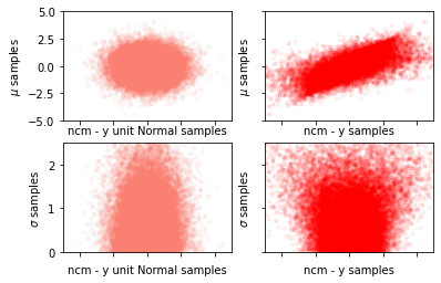
def noncentered_model():
# generate data
np.random.seed(0)
n = 1
m = 10000
mu = norm.rvs(0, 3, m)
sigma = halfnorm.rvs(0, 2, m)
y = norm.rvs(mu, sigma, (n, m))
# set up model
with pm.Model():
mu_ = pm.Normal("mu", 0, 1)
sigma_ = pm.HalfNormal("sigma", 1)
yt_ = pm.Normal("yt", 0, 1, shape=n)
pm.Deterministic("y", mu_ + yt_ * sigma_)
# y_ = pm.Normal("y", mu_, sigma_, shape=n)
# sample and save samples
trace = pm.sample(m, chains=3)
mu_samples = trace["mu"][:]
sigma_samples = trace["sigma"][:]
yt_samples = trace["yt"].T[:]
y_samples = trace["y"].T[:]
# plot 2-D figures
sc = 5
fig, axes = plt.subplots(2, 2, constrained_layout=False, sharex=True)
ax = axes[0, 0]
ax.scatter(yt_samples[0], mu_samples, marker=".", alpha=0.05, rasterized=True, color="salmon")
ax.set_xlim(-sc, sc)
ax.set_ylim(-sc, sc)
ax.set_ylabel("$\mu$ samples")
ax.set_xlabel("ncm - y unit Normal samples")
ax.set_xticklabels([])
ax = axes[0, 1]
ax.scatter(y_samples[0], mu_samples, marker=".", alpha=0.05, rasterized=True, color="r")
ax.set_xlim(-sc, sc)
ax.set_ylim(-sc, sc)
ax.set_ylabel("$\mu$ samples")
ax.set_xlabel("ncm - y samples")
ax.set_yticklabels([])
ax.set_xticklabels([])
ax = axes[1, 0]
ax.scatter(yt_samples[0], sigma_samples, marker=".", alpha=0.05, rasterized=True, color="salmon")
ax.set_xlim(-sc, sc)
ax.set_ylim(0, sc / 2)
ax.set_xlabel("ncm - y unit Normal samples")
ax.set_ylabel("$\sigma$ samples")
ax = axes[1, 1]
ax.scatter(y_samples[0], sigma_samples, marker=".", alpha=0.05, rasterized=True, color="r")
ax.set_xlim(-sc, sc)
ax.set_ylim(0, sc / 2)
ax.set_yticklabels([])
ax.set_xlabel("ncm - y samples")
ax.set_ylabel("$\sigma$ samples")
plt.show()
return(trace)
trace_cm = centered_model()
trace_ncm = noncentered_model()
/Users/srijith.rajamohan/opt/anaconda3/envs/pymc3nightly_env/lib/python3.9/site-packages/pymc3/sampling.py:465: FutureWarning: In an upcoming release, pm.sample will return an `arviz.InferenceData` object instead of a `MultiTrace` by default. You can pass return_inferencedata=True or return_inferencedata=False to be safe and silence this warning.
  warnings.warn(
Auto-assigning NUTS sampler...
Initializing NUTS using jitter+adapt_diag...
Multiprocess sampling (3 chains in 4 jobs)
NUTS: [y, sigma, mu]
Sampling 3 chains for 1_000 tune and 10_000 draw iterations (3_000 + 30_000 draws total) took 15 seconds.
There were 2027 divergences after tuning. Increase `target_accept` or reparameterize.
The acceptance probability does not match the target. It is 0.6613714331625662, but should be close to 0.8. Try to increase the number of tuning steps.
There were 1543 divergences after tuning. Increase `target_accept` or reparameterize.
The acceptance probability does not match the target. It is 0.7064652733253344, but should be close to 0.8. Try to increase the number of tuning steps.
There were 3741 divergences after tuning. Increase `target_accept` or reparameterize.
The acceptance probability does not match the target. It is 0.5066897639865938, but should be close to 0.8. Try to increase the number of tuning steps.
The rhat statistic is larger than 1.05 for some parameters. This indicates slight problems during sampling.
The estimated number of effective samples is smaller than 200 for some parameters.
/Users/srijith.rajamohan/opt/anaconda3/envs/pymc3nightly_env/lib/python3.9/site-packages/pymc3/sampling.py:465: FutureWarning: In an upcoming release, pm.sample will return an `arviz.InferenceData` object instead of a `MultiTrace` by default. You can pass return_inferencedata=True or return_inferencedata=False to be safe and silence this warning.
  warnings.warn(
Auto-assigning NUTS sampler...
Initializing NUTS using jitter+adapt_diag...
Multiprocess sampling (3 chains in 4 jobs)
NUTS: [yt, sigma, mu]
Sampling 3 chains for 1_000 tune and 10_000 draw iterations (3_000 + 30_000 draws total) took 13 seconds.
There were 9 divergences after tuning. Increase `target_accept` or reparameterize.
There were 69 divergences after tuning. Increase `target_accept` or reparameterize.
There were 79 divergences after tuning. Increase `target_accept` or reparameterize.
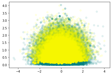
plt.figure()
plt.scatter(trace_ncm['mu'], trace_ncm['sigma'],c='teal', alpha=0.1)
plt.scatter(trace_cm['mu'], trace_cm['sigma'], c='yellow', alpha=0.1)
plt.show()
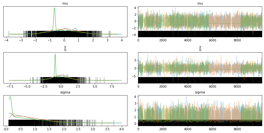
Convergence
import arviz as az
print("------------ Centered model ------------")

# The bars indicate the location of the divergences in the sampling process
az.plot_trace(trace_cm, divergences='bottom')
az.summary(trace_cm)
------------ Centered model ------------
/Users/srijith.rajamohan/opt/anaconda3/envs/pymc3nightly_env/lib/python3.9/site-packages/arviz/data/io_pymc3.py:87: FutureWarning: Using `from_pymc3` without the model will be deprecated in a future release. Not using the model will return less accurate and less useful results. Make sure you use the model argument or call from_pymc3 within a model context.
  warnings.warn(
| mean | sd | hdi_3% | hdi_97% | mcse_mean | mcse_sd | ess_mean | ess_sd | ess_bulk | ess_tail | r_hat | |
|---|---|---|---|---|---|---|---|---|---|---|---|
| mu | -0.095 | 0.970 | -1.865 | 1.820 | 0.042 | 0.030 | 535.0 | 535.0 | 578.0 | 554.0 | 1.01 |
| y[0] | -0.109 | 1.406 | -2.795 | 2.447 | 0.046 | 0.033 | 931.0 | 931.0 | 804.0 | 782.0 | 1.01 |
| sigma | 0.791 | 0.586 | 0.095 | 1.861 | 0.050 | 0.036 | 135.0 | 135.0 | 50.0 | 9.0 | 1.06 |
print("------------ Non-centered model ------------")

# The bars indicate the locations of divergences in the sampling process
az.plot_trace(trace_ncm, divergences='top')
az.summary(trace_ncm)
------------ Non-centered model ------------
/Users/srijith.rajamohan/opt/anaconda3/envs/pymc3nightly_env/lib/python3.9/site-packages/arviz/data/io_pymc3.py:87: FutureWarning: Using `from_pymc3` without the model will be deprecated in a future release. Not using the model will return less accurate and less useful results. Make sure you use the model argument or call from_pymc3 within a model context.
  warnings.warn(
| mean | sd | hdi_3% | hdi_97% | mcse_mean | mcse_sd | ess_mean | ess_sd | ess_bulk | ess_tail | r_hat | |
|---|---|---|---|---|---|---|---|---|---|---|---|
| mu | -0.001 | 1.005 | -1.902 | 1.851 | 0.007 | 0.006 | 21283.0 | 14008.0 | 21272.0 | 17802.0 | 1.0 |
| yt[0] | 0.008 | 1.009 | -1.851 | 1.901 | 0.008 | 0.006 | 17563.0 | 14233.0 | 17563.0 | 17653.0 | 1.0 |
| sigma | 0.812 | 0.604 | 0.000 | 1.903 | 0.005 | 0.003 | 16672.0 | 16672.0 | 12311.0 | 9148.0 | 1.0 |
| y[0] | 0.014 | 1.429 | -2.635 | 2.732 | 0.011 | 0.008 | 18363.0 | 16850.0 | 18828.0 | 17084.0 | 1.0 |
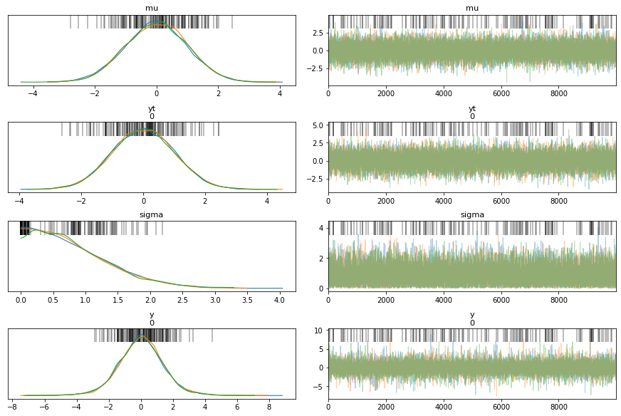
The posterior densities have more agreement for the non-centered model(ncm) compared to the centered model (cm), for the different chains.
There are more divergences for centered model compared to the non-centered model as can be seen from the vertical bars in the trace plot.
In general, the non-centered model mixes better than the centered model - non-centered model looks fairly evenly mixed while centered model looks patchy in certain regions.
It is possible to see flat lines in the trace for a centered model, a flat line indicates that the same sample value is being used because all new proposed samples are being rejected, in other words the sampler is sampling slowly and not getting to a different space in the manifold. The only fix here is to sample for longer periods of time, however we are assuming that we can get more unbiased samples if we let it run longer.
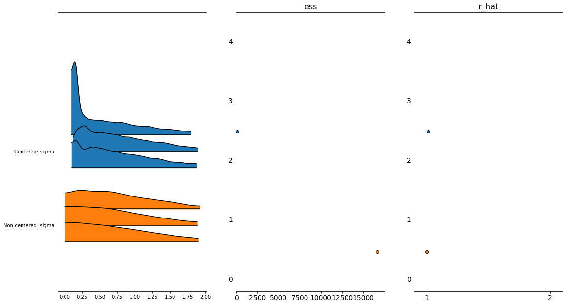
Forest Plot
We plot the densities of both the cm and the ncm models, notice the differences in effective sample sizes for the centered model (very low).
fig, axs = plt.subplots(1,3)
fig.set_size_inches(18.5, 10.5)
az.plot_forest([trace_cm, trace_ncm], var_names=['sigma'],
               kind = 'ridgeplot',
               model_names=['Centered','Non-centered'],
               combined=False,
               ess=True,
               r_hat=True,
               ax=axs[0:3],
               figsize=(20,20) )
#az.plot_forest(trace_ncm, var_names=['a'],
#               kind='ridgeplot',
#               combined=False,
#               ess=True,
#               r_hat=True,
#               ax=axs[1,0:3])
/Users/srijith.rajamohan/opt/anaconda3/envs/pymc3nightly_env/lib/python3.9/site-packages/arviz/data/io_pymc3.py:87: FutureWarning: Using `from_pymc3` without the model will be deprecated in a future release. Not using the model will return less accurate and less useful results. Make sure you use the model argument or call from_pymc3 within a model context.
  warnings.warn(
array([<AxesSubplot:>, <AxesSubplot:title={'center':'ess'}>,
       <AxesSubplot:title={'center':'r_hat'}>], dtype=object)
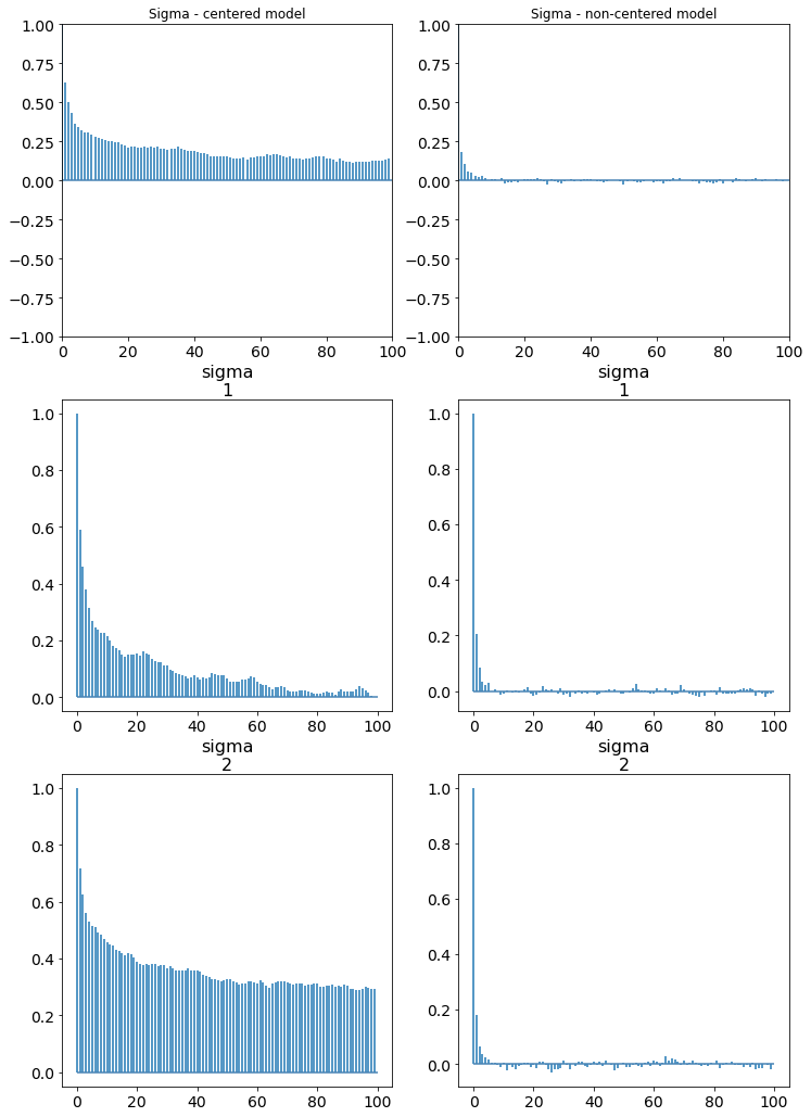
Autocorrelation and effective sample sizes
Ideally, we would like to have zero correlation in the samples that are drawn. Correlated samples violate our condition of independence and can give us biased posterior estimates of our posterior distribution. Thinning or pruning refers to the process of dropping every nth sample from a chain. This is to minimize the number of correlated samples that might be drawn, especially if the proposal distribution is narrow. The autocorrelation plot computes the correlation of a sequence with itself but shifted by n; for each n on the x axis the corresponding value of autocorrelation is plotted on the y axis.
az.plot_autocorr(trace, var_names=["a", "b"])
Techniques like Metropolis-Hastings are susceptible to having auto-correlated samples. We plot the autocorrelation here for the cm and the ncm models. The cm models have samples that have a high degree of autocorrelation while the ncm models does not.
fig, axs = plt.subplots(3,2)
fig.set_size_inches(12, 18)
az.plot_autocorr(trace_cm, var_names=['sigma'], ax=axs[0:3,0])
az.plot_autocorr(trace_ncm, var_names=['sigma'], ax=axs[0:3,1])
axs[0][0].set_title('Sigma - centered model')
axs[0][1].set_title('Sigma - non-centered model')
/Users/srijith.rajamohan/opt/anaconda3/envs/pymc3nightly_env/lib/python3.9/site-packages/arviz/data/io_pymc3.py:87: FutureWarning: Using `from_pymc3` without the model will be deprecated in a future release. Not using the model will return less accurate and less useful results. Make sure you use the model argument or call from_pymc3 within a model context.
  warnings.warn(
Text(0.5, 1.0, 'Sigma - non-centered model')
Since a chain with autocorrelation has fewer samples that are independent, we can calculate the number of effective samples called the effective sample size. This is listed when a summary of the trace is printed out, however it can also be explicitly computed using
az.effective_n(trace_s)
PyMC3 will throw a warning if the number of effective samples is less than 200 (200 is heuristically determined to provide a good approximation for the mean of a distribution). Unless you want to sample from the tails of a distribution (rare events), 1000 to 2000 samples should provide a good approximation for a distribution.
Monte Carlo error
The Monte Carlo error is a measure of the error of our sampler which stems from the fact that not all samples that we have drawn are independent. This error is defined by dividing a trace into ‘n’ blocks. We then compute the mean of these blocks and calculate the error as the standard deviation of these means over the square root of the number of blocks.
\(mc_{error} = \sigma(\mu(block_i)) / \sqrt(n)\)
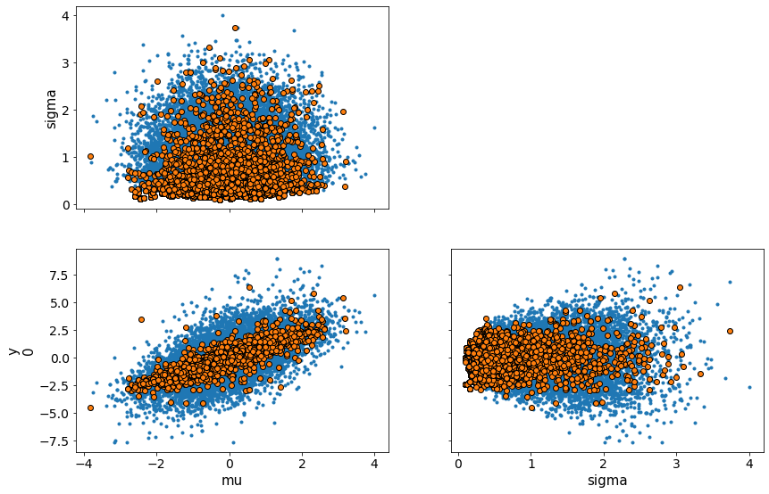
Divergence
Divergences happen in regions of high curvature or high gradient in the manifold. When PyMC3 detects a divergence it abandons that chain, and as a result the samples that are reported to have been diverging are close to the space of high curvature but not necessarily right on it.
In some cases, PyMC3 can indicate falsely that some samples are divergences, this is due to the heuristics used to identify divergences. Concentration of samples in a region is an indication that these are not divergences.
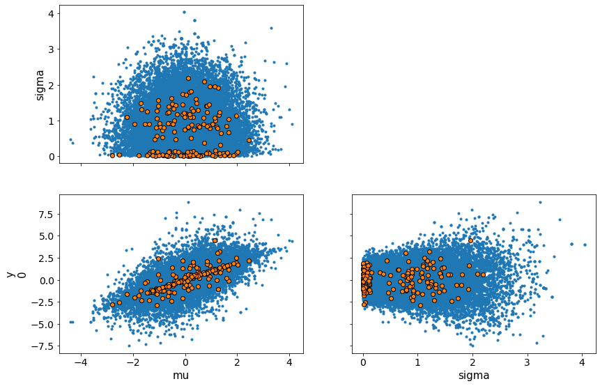
We visualize this for the cm and ncm models with pairplots of the variables. You can see how the cm models have difficulty sampling at the edge of the funnel shaped two-dimensional manifold formed by the pairplot.
# Get the divergences
print("Number of divergences in cm model, %d and %lf percent " % (trace_cm['diverging'].nonzero()[0].shape[0], trace_cm['diverging'].nonzero()[0].shape[0]/ len(trace_cm) * 100))
divergent = trace_cm['diverging']

print("Number of divergences in ncm model, %d and %lf percent " % (trace_ncm['diverging'].nonzero()[0].shape[0], trace_ncm['diverging'].nonzero()[0].shape[0]/ len(trace_ncm) * 100))
divergent = trace_cm['diverging']
Number of divergences in cm model, 7311 and 73.110000 percent
Number of divergences in ncm model, 157 and 1.570000 percent
Pairplots
print("Centered model")
az.plot_pair(trace_cm, var_names = ['mu', 'sigma', 'y'], divergences=True)
Centered model
/Users/srijith.rajamohan/opt/anaconda3/envs/pymc3nightly_env/lib/python3.9/site-packages/arviz/data/io_pymc3.py:87: FutureWarning: Using `from_pymc3` without the model will be deprecated in a future release. Not using the model will return less accurate and less useful results. Make sure you use the model argument or call from_pymc3 within a model context.
  warnings.warn(
array([[<AxesSubplot:ylabel='sigma'>, <AxesSubplot:>],
       [<AxesSubplot:xlabel='mu', ylabel='y\n0'>,
        <AxesSubplot:xlabel='sigma'>]], dtype=object)
print("Non-centered model")
az.plot_pair(trace_ncm, var_names = ['mu', 'sigma', 'y'], divergences=True)
Non-centered model
/Users/srijith.rajamohan/opt/anaconda3/envs/pymc3nightly_env/lib/python3.9/site-packages/arviz/data/io_pymc3.py:87: FutureWarning: Using `from_pymc3` without the model will be deprecated in a future release. Not using the model will return less accurate and less useful results. Make sure you use the model argument or call from_pymc3 within a model context.
  warnings.warn(
array([[<AxesSubplot:ylabel='sigma'>, <AxesSubplot:>],
       [<AxesSubplot:xlabel='mu', ylabel='y\n0'>,
        <AxesSubplot:xlabel='sigma'>]], dtype=object)
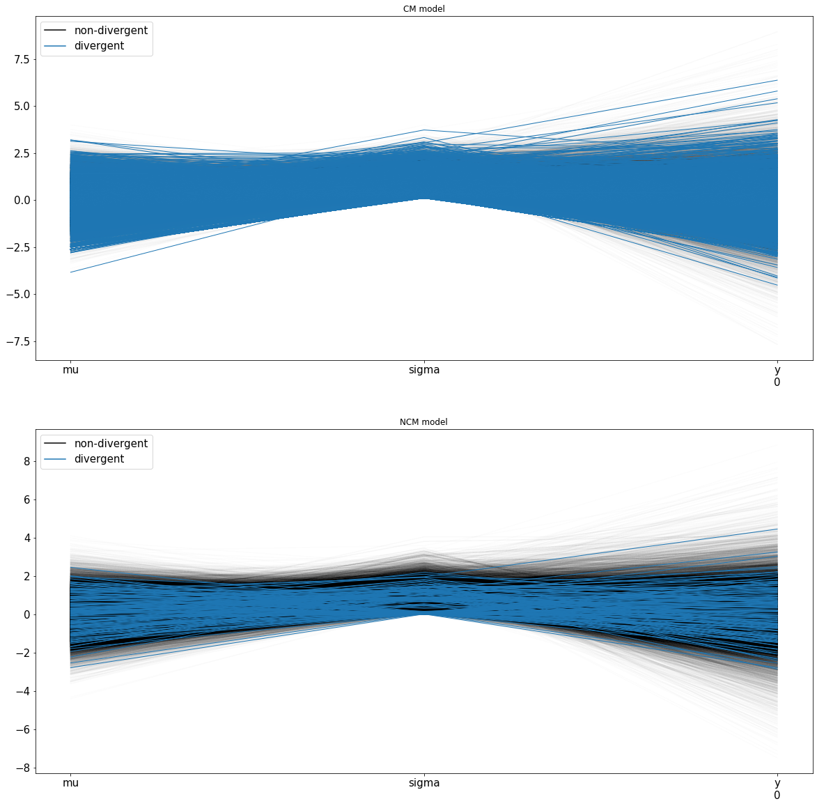
Parallel Coordinates
You can also have a parallel coordinates plot of the variables to look at the multidimensional data instead of pairplots. If we notice tight-knit lines around a region, that is an indication of difficulty sampling and hence divergences. This behavior can be observed in the centered model around 0 while the non-centered model has a sparser cluster of lines around 0. Sparser clusters can be an indication of false positives where divergences are reported. Apart from reformulating the problem, there are two ways to avoid the problem of divergences.
Increase the tuning samples
Increase ‘target_accept’
The parallel coordinates below show a much denser set of lines for the divergences for the centered model.
fig, axs = plt.subplots(2,1)
fig.set_size_inches(20,20)
axs[0].set_title('CM model')
axs[1].set_title('NCM model')
az.plot_parallel(trace_cm, var_names=['mu','sigma','y'], figsize=(20,20), shadend=0.01, colord='tab:blue', textsize=15, ax=axs[0])
az.plot_parallel(trace_ncm, var_names=['mu','sigma','y'], figsize=(20,20), shadend=0.01, colord='tab:blue', textsize=15,ax=axs[1])
/Users/srijith.rajamohan/opt/anaconda3/envs/pymc3nightly_env/lib/python3.9/site-packages/arviz/data/io_pymc3.py:87: FutureWarning: Using `from_pymc3` without the model will be deprecated in a future release. Not using the model will return less accurate and less useful results. Make sure you use the model argument or call from_pymc3 within a model context.
  warnings.warn(
<AxesSubplot:title={'center':'NCM model'}>
A note on why we compute the log of the posterior
In short, this is done to avoid numerical overflow or underflow issues. When dealing with really large or small numbers, it is likely the limited precision of storage types (float, double etc.) can be an issue. In order to avoid this, the log of the probabilities are used instead in the calculations.