Setting up Your Python Environment
There are a few ways you can set up your Python environment for the notebooks that are going to be used for the courses here.
The notebooks can be downloaded from each course page by clicking the tab on the top right corner and selecting ‘.ipynb’.
Databricks Community Edition
Databricks offers a Community Edition of their Data Science ecosystem for running experiments in notebooks. You can sign up for a free account and start running the notebooks for the course. The advantages of using Databricks over other Data Science ecosystems:
Integration with MLflow for experiment management
Integration with Git for version control of your notebooks
Integration with your AWS, GCP and Azure accounts if you so desire
Easy to setup a cluster for scaling your Data Science workflows
Collaborate and comment on notebooks with your team
Easily publish your notebooks for public consumption
Binder
Once you are on a course page that has a Jupyter Notebook, click on the tab located at the top right corner of the page and select ‘Binder’. This deploys the notebook onto a cloud environment. Binder automatically pulls the Docker image and creates a working Python environment for you without any user intervention. This is the easiest way to get started using the notebooks. However, any changes made in the notebooks will not be persistent. If persistence is desired, it is recommended to use the Databricks Community Edition.
Anaconda
The preferred Python distribution is
Anaconda. Anaconda is a cross-platform distribution that has a fairly comprehensive set of packages. Anaconda comes with a package management system called conda to organize
your environment.
Jupyter Notebooks
Jupyter notebooks offer an integrated and intuitive enviroment for rapid prototyping, teaching and presenting Data Science and Scientific Computing applications written in Python, R and Julia (although there is growing suport for additional languages such as C++).
It uses a browser-based interface with the following capabilities (not comprehensive)
The ability to write and execute Python commands.
Formatted output in the browser, including tables, figures, animation, etc.
The option to mix in formatted text and mathematical expressions.
Figure %s shows the execution of some code (borrowed from
here)
in a Jupyter notebook
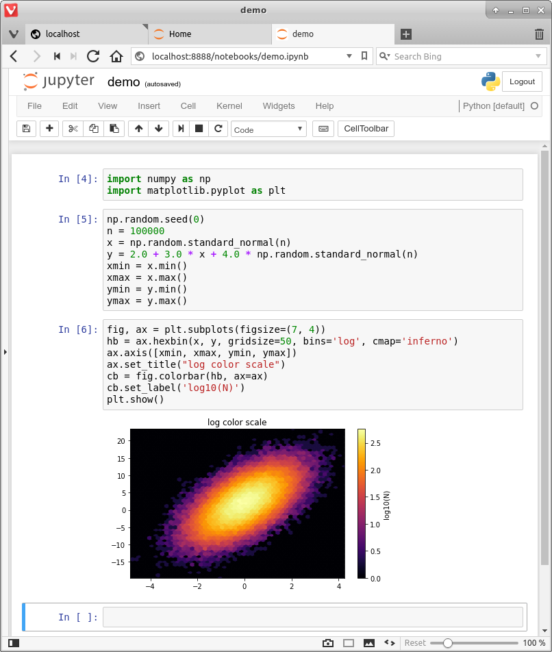
Fig. 1 A Jupyter notebook viewed in the browser
Starting the Jupyter Notebook
Once you have installed Anaconda, you can start the Jupyter notebook.
Either
search for Jupyter in your applications menu, or
open up a terminal and type
jupyter notebookWindows users should substitute “Anaconda command prompt” for “terminal” in the previous line.
If you use the second option, you will see something like this
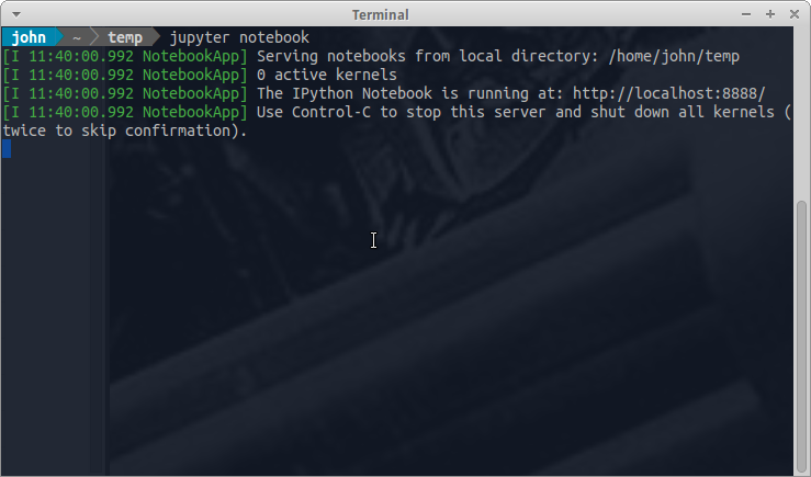
The output tells us the notebook is running at http://localhost:8888/
localhostis the name of the local machine8888refers to port number 8888 on your computer
Thus, the Jupyter kernel is listening for Python commands on port 8888 of our local machine.
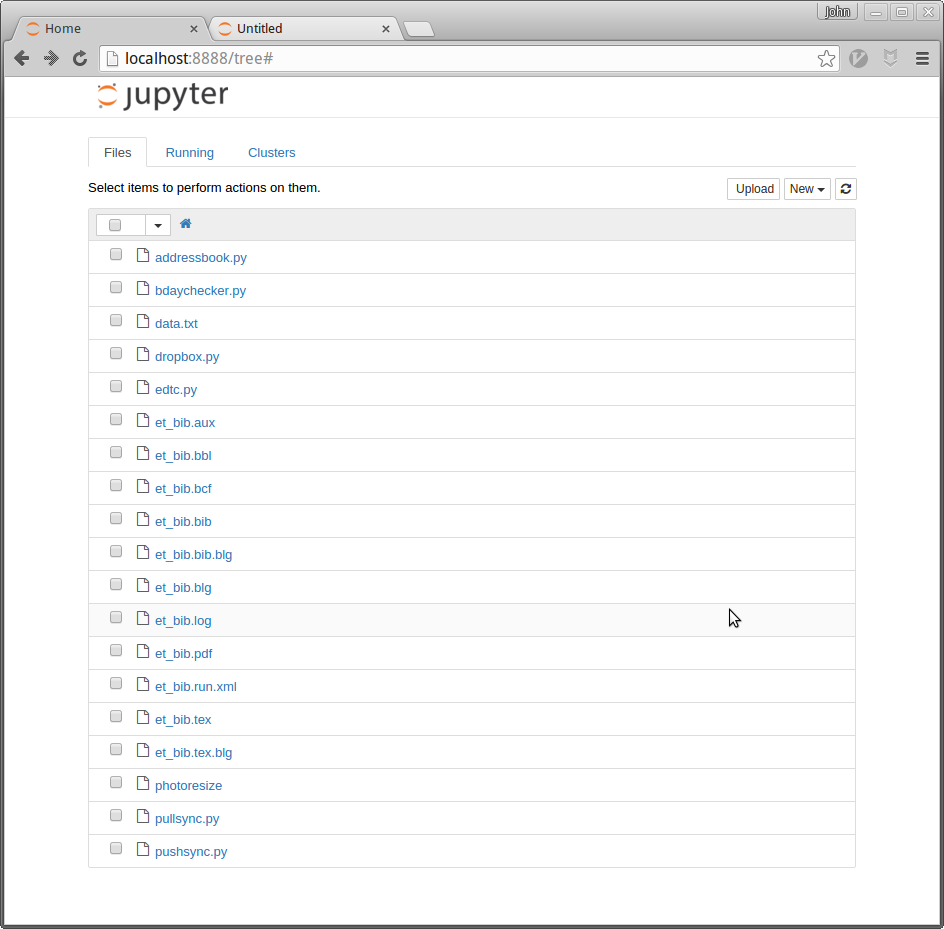
Hopefully, your default browser has also opened up with a web page that looks something like this