Distributions, central tendency, and shape parameters¶

In the last video, we discussed sample spaces, events and probability spaces. We looked at rules for addition and multiplication of probabilities which follow directly from the Axioms of Probability (Kolmogorov Axioms). Here we will continue and extend that discussion to probability distributions and descriptions of those distributions.

Our topics include:

probability distributions (discrete vs continuous, pmf vs pdf).
moments, expectations and variances.
joint distributions, expectations and covariances with 2 variables.
marginals.

General references:

Statistical Inference (9780534243128): Casella, George, Berger, Roger L.
Probability Theory and Statistical Inference: Empirical Modeling with Observational Data (9781107185142): Spanos, A.
Bayesian Models: A Statistical Primer for Ecologists (9780691159287): Hobbs, N. Thompson, Hooten, Mevin B.
A First Course in Bayesian Statistical Methods (0387922997): Hoff, Peter D.

Probability distributions¶

As a reminder, last time we had introduced the concept of a probability space as a combination of a sample space, event space, and probability function. The probability function is a real-valued function mapping events to the interval [0,1]. The probability function adheres to the Axioms of Probability (Kolmogorov Axioms). These are summarized as:

the probability of an event is a real number on the interval [0,1]

\[0 \le P(E) \le 1\]
the probability of at least one event occurring is 1

\[P(S) = 1\text{, where S is the sample space}\]
countable mutually exclusive sets of events satisfy the following

\[P(\bigcup_{i=1}^\infty E_i) = \sum_{i=1}^\infty P(E_i)\]

In addition to the probability space, we talked about random variables being (often) real-valued functions mapping outcomes (really events) to a measurable space. In set notation, this looks like:

\[X: \Omega \to \mathbb{R}\]

Combining the mapping of events with the association of the probability function, we have what we need to study random processes. This mapping defines the probability given by X in a measurable set as:

\[P(X \in S) = P({x \in \Omega | X(x) \in S})\]

For example, consider the case of tossing two fair coins where we are interested in the events being {(HH),(TT)} or not. Our sample space is:

\[S = \{(HH),(TT),(TH),(HT)\}\]

Our event space is:

$\mathcal{F} = {S, \bar{S}, E, \bar{E} }$, where we have defined $E = {(HH),(TT)}$

If we define X(HH)=X(TT)=1, 0 otherwise, we get to:

\[\begin{split}P_X(x) = \begin{cases} \frac{1}{2}, \text{for x = 1} \\ \frac{1}{2}, \text{for x = 0} \\ \end{cases} \end{split}\]

We now have our first random variable which happens to be distributed according to the Bernoulli distribution more generally given as:

$X \sim Bern(\theta)$, where

\[\begin{split}f(x;\theta) = P(X=x;\theta) = \begin{cases} \theta, \text{for x = 1} \\ 1 - \theta, \text{for x = 0} \\ \end{cases} \end{split}\]

\[f(x;\theta) = \theta^x(1-\theta)^{(1-x)}\]

For $\theta$ = [0,1]. Distributions are associated with parameters. As defined above, we see $\theta$ as the parameter associated with the Bernoulli distribution is the probability of success.

Discrete random variables¶

As above, discrete random variables are characterized by countable outcome spaces. Discrete random variables are associated with a probability mass function (pmf) whose range is a countable subset of $\mathbb{R}$ with probability values in the range [0,1]. Properties of the pmf include:

$f_x(x) \ge 0$, for all $x \in \mathbb{R}_X$.
$\sum_{x \in X} f_x(x) = 1$
$F_X(b) - F_X(a) = \sum_{x=a}^b f(x), a < b, a, b \in \mathbb{R}$

The last property involves the cdf (cumulative distribution function). The cdf is defined such that:

$F_X(b) = \sum_{x \in [-\infty,b]} f_X(x)$

Which, with some thought, we could come up with the properties of the cdf:

non-decreasing: $F_X(x) \le F_X(y)$, for all $x \le y$
right-continuous: $\lim_{x \downarrow x_0^+} F_X(x) = F_X(x_0)$
positive, with range [0,1]

For discrete variables, $F_X(x) = P(X \le x) = \sum_{x_i \le x}f(x_i)$

Continuous random variables¶

In the discrete case, random variables are characterized by countable outcome spaces where the random variable maps events to discrete values on $\mathbb{R}$. How do we deal with outcome spaces that are continuous? We use intervals.

Continuous random variables are associated with a probability density function (pdf) whose range is an uncountable subset of $\mathbb{R}$ with probability values in the range [0,$\infty$]. Properties of the pdf include:

$f_x(x) \ge 0$, for all $x \in \mathbb{R}_X$.
$\int_{-\infty}^\infty f_x(x)dx = 1$
$F_X(b) - F_X(a) = \int_{a}^b f(x)dx,\ a < b, (a, b) \in \mathbb{R}$

Note, the cdf of a continuous random variable is generally defined as: $P(X \le x) = F_X(x) = \int_{-\infty}^x f(u)du$ where we can we can recover the pdf via $f(x) = \frac{dF(x)}{dx}$. The properties of the continuous cdf are obvious extensions of the discrete case. One difference we sometimes overlook is the $P(X=x)=0$ in the continuous case because $x$ is a point value. To solve this conundrum, we we use intervals, ie area under the curve when talking probabilities.

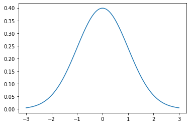
Without derivation, the most widely studied and used distribution in statistics is the normal distribution. The pdf of the normal distribution is given as

\[X \sim Norm(\mu,\sigma^2) \text{, where}\]

\[f_x(x,\mu,\sigma^2) = \frac{1}{\sqrt{2\pi\sigma^2}}e^{-\frac{(x-\mu)^2}{2\sigma^2}}, (x,\mu,\sigma^2) \in (\mathbb{R},\mathbb{R},\mathbb{R}_+)\]

A plot of the pdf is show below. Where we are setting $\mu = 0$ and $\sigma^2=1$. Note, the parameters of the distribution as given are $\mu$ and $\sigma^2$. The parameters of the normal distribution describe the shape: $\mu$ gives the center of mass while $\sigma^2$ gives an indication of spread.

import matplotlib.pyplot as plt
import numpy as np
import scipy.stats as stats
import math

mu = 0
variance = 1
sigma = math.sqrt(variance)
x = np.linspace(mu - 3*sigma, mu + 3*sigma, 100) #bounds and granularity
plt.plot(x, stats.norm.pdf(x, mu, sigma))
plt.show()

../../_images/Fundamentals-lecture3-intro-distributions-unGRADED_4_0.png

Moments, expectations and variances¶

Distributions are recognizable by characteristics such as range, location and shape. Computing moments such as expectation, variance, skewness and kurtosis can be used to estimate the parameters that define a distribution.

Expectation¶

The expectation of a function is the average value of the function under a probability distribution. In the case of discrete distributions, this is computed as the weighted average where the weights are dictated by the probability at the value of x (where p(x) is the pmf/pdf):

\[E[f] = \sum_x f(x)^r p(x)\]

For continuous distributions, this looks like

\[E[f] = \int f(x)^r p(x) dx.\]

if $f(x) = x$ and $r=1$ in both cases, this is called the mean of the distribution. In the figure of the normal distribution above, computing the expectation will give $E[x]=0$ which matches our intuition of where the bulk of the mass is centered based on the figure.

For the Bernoulli distribution given earlier, we compute this as

\[E[x] = \sum_{x=0,1} x\ast p(x,\theta) = 0\ast(1-\theta) + 1\ast\theta = \theta\]

Thus, for the Bernoulli distribution, the mean is equal to the parameter for success, $E[x]_{Bern} = \theta$.

Variance, skewness, kurtosis¶

While the mean of the distribution, also the first raw moment, is given by the first power of $x^1$, other interesting moments arise when we take powers of $X-E[X]$.

Variance, measures spread of the distribution:
$$Var(X) = E[(X-E[X])^2] = \int (X-E[X])^2 p(x) dx\text{ in the continuous case}$$

Skewness, measures symmetry:
$$\alpha_3 = \frac{E(X-E[X])^3}{(\sqrt{Var(X)})^3}$$

Kurtosis, measures “peakiness”:
$$\alpha_4 = \frac{E(X-E[X])^4}{(\sqrt{Var(X)})^4}$$

Properties of mean and variance¶

Expectation is a linear operator. As such, we can easily prove the following useful properties:

$E[c] = c$, where c is a constant.
$E[aX_1 + bX_2] = aE[X_1] + bE[X_2]$

Similarly, with variance:

$Var(X) = E[(X-E[X])^2] = E[X^2] - (E[X])^2$
$Var(c) = 0$, where c is a constant.
$Var(aX_1 + bX_2) = a^2Var(X_1) + b^2Var(X_2)$

Standard deviation is $\sqrt{Var(X)}$. This is a useful quantity as it is on the same scale as X.

Other measures¶

Mode – most frequent value. $\frac{df(x)}{dx}=0$ needs to be max.

Median – middle value, place where probability is equal to right/left. $P(X < x) = P(X > x) = 1/2$

Quantiles are defined using the cdf. $F_X(x) \ge p$

For the normal distribution, mean = median = mode.

Joint distributions¶

In many cases, we will be working on distributions of more than one variable. These are termed joint distributions. These joint distributions can be of mixed type, eg Bernoulli and normal, normal and Cauchy, etc. These can be thought of in the normal way:

\[P_{XY}(x,y) = P(X=x,Y=y)\]

We often want to determine a parameter in a distribution of more than one variable. For instance, the expectation of $f(x,y)$

\[E[f(x,y)] = \int_{x,y} f(x,y) p(x,y) dxdy\]

where $f(x,y)=xy$ would give the mean analogous to the univariate case.

Marginal distribution¶

In cases where we have a joint distribution, we will sometimes need to find the marginal distribution. The marginial distribution for a case where we have a joint distribution of X and Y is:

$P_X(x) = \sum_{all y_i} P_{XY}(x,y_i)$ and simularly for the marginal in Y. The extension to a continuous case or mixed case is an obvious use of an integral.

Intuitively, we are integrating (or averaging) out the effect of R.V. Y to get at the marginal distribution of X.

Conditional distributions¶

Remember our rules of probability …

\[P_{XY}(x_i|y_j) = \frac{P_{XY}(x_i,y_j)}{P_Y(y_i)}\]

The conditional expectation is given by

\[E[X|Y=y_j] = \sum_{X} x_iP_{X|Y}(x_i|y_j)\]

or in the continuous case for a function g:

\[E[g(Y)|x] = \int_{-\infty}^{\infty} g(y)f(y|x)dy\]

Independence¶

It can be shown that if X and Y are independent, there exists some functions g(x) and h(y) such that:

\[f(x,y) = g(x)h(y)\text{ for all (x,y)}\]

How do we use this? In the discrete case, if we can find a pair (x,y) that violate the product rule, the random variables are dependent.

Covariance¶

\[cov[x,y] = E[(x-E[x])(y-E[y])] = E_{x,y}[xy]-E_x[x]E_y[y]\]

Correlation (correlation coefficient)¶

The correlation coefficient gives an indication of how much or little X,Y vary together. If X,Y are independent, $cov(X,Y)= corr(X,Y) = 0$. The corollary is not necessarily true. $$\rho_{XY} = \frac{Cov(X,Y)}{\sigma_x\sigma_y}$$

GRADED EVALUATION (15 mins)¶

Are X and Y independent?

\[f(x,y) = \frac{1}{57}xy^6e^{-y-x},x>0,y>0\]

a. True
b. False

\[\]

The marginal distribution of X

\[f(x,y) = 4xy; x,y \in [0,1]\]

a. is a function of x
b. is a function of y